Non-Inverting Op-Amp Analysis with Time Constants

The seminal paper by Hajimiri on analyzing circuits using time constant techniques, such the zero-value and infinite-value time constants based on the Cochrun-Grabel method allows an easy analysis by breaking a complicated network into smaller parts.

The technique is based on opening and shorting dynamic elements such that the analysis of different terms in an standard transfer function are filled in term by term:

$$\begin{aligned} H(s)=\frac{a_0 + a_1s+a_2s^2+\cdots}{1+b_1s+b_2s^2+\cdots} \end{aligned}$$

Hajimiri’s paper already provides instructive examples of several passive and active circuits (i.e. circuits with dependent sources). This article intends to also show that this method can be applied to the analysis of op-amps, assuming a simple finite gain op-amp.

Non-Inverting Op-Amp Closed-Loop Gain

$$\begin{aligned} H(s)=\frac{a_0 + a_1s}{1+b_1s} \end{aligned}$$

$$\begin{aligned} a_0 = \frac{R_g + R_f}{R_g}\\ b_1 = \tau_{C_f} = C_fR_f \\ a_1 = 1\tau_{C_f} \end{aligned}$$

How did we derive each term in the laplace expression?

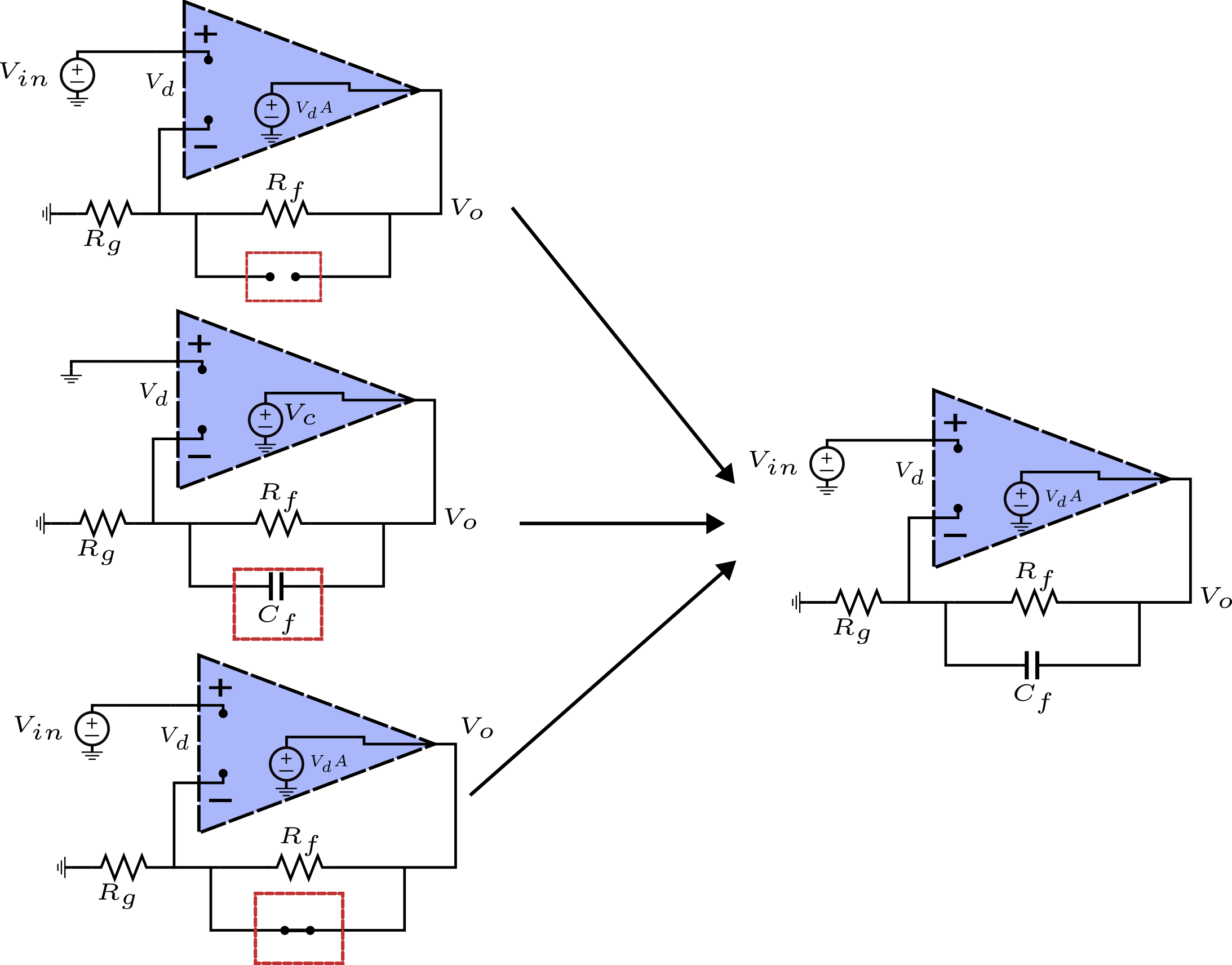
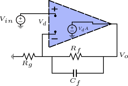
• $a_0:$ This is the zero-value time constant. In this case, this equals the standard non-inverting op amp transfer function. Therefore, all dynamic elements will be set to their DC value ($C_f$ will be an open).
  
• $b_1:$ This is the zero-value time constant related to $C_f$.Under the assumption of an ideal op-amp (i.e. V(+) = V(-)), the top side of $R_g$ is grounded as well; it’s, effectively, out of the picture. Therefore, the only resistance seen by $C_f$ is $R_f$.
  
• $a_1:$ This is the transfer from input to output assuming $C_f$ is infinite-valued (i.e. it becomes a short). When doing so, we can recognize that the non-inverting voltage amplifier, effectively, degenerates into a simple voltage buffer; $R_g$ doesn’t matter. Hence, this transfer is equal to 1. This factor must be multiplied, now, by the time constant associated with the dynamic element (i.e. $C_f$) that infinite-valued.
  

Finally, we can write the closed-loop gain formula as:

$$\begin{aligned} H(s)=\frac{\frac{R_g+R_f}{R_g} + C_fR_fs}{1+C_fR_fs} \end{aligned}$$

However, it might be more intuitive to factor out the low-frequency gain as follows:

$$\begin{aligned} H(s)=\left(1+\frac{R_f}{R_g}\right)\frac{1+C_f\frac{R_fR_g}{R_f+R_g}s}{1+C_fR_fs} = \left(1+\frac{R_f}{R_g}\right)\frac{1+C_f(R_f||R_g)s}{1+C_fR_fs} \end{aligned}$$

Non-Inverting Op-Amp Loop Gain

This is loop gain formula will be of 1st order as well: $$\begin{aligned} L = \frac{V_d}{AV_c} = \frac{a_0 + a_1s}{1+b_1s} \end{aligned}$$

$$\begin{aligned} a_0 = \frac{R_g}{R_g + R_f}\\ b_1 = \tau_{C_f} = C_f(R_f||R_g)\\ a_1 = \tau_{C_f} = C_f(R_f||R_g)\ \end{aligned}$$

How did we derive each term in the loop gain formula?

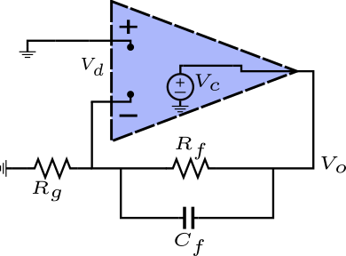
• $a_0:$ All dynamic elements are set to their DC value (i.e. $C_f$ is an open). Therefore, it is easy to see that the transfer from $V_c$ to $V_d$ is a simply voltage divider by $R_g$ and $R_f$.
  
• $b_1:$ Since there’s only one dynamic element (i.e. $C_f$), we turn off all inputs (in this case, $V_c$, which would be shorted to ground.) and simply calculate the impedance seen by $C_f$. Since $R_f$ is grounded on its right side, then it is effectively in parallel with $R_g$.
  
• $a_1:$ This is the transfer from $V_c$ to $V_d$ while setting $C_f$ to its infinite value (i.e. a short). As a consequence, the voltage divider due to $R_g$ and $R_f$ becomes useless, because $R_f$ is now shorted. Therefore, the transfer is simply 1. This transfer factor must be multiplied by the time constant of $C_f$, because we infinite-valued it.
  

Therefore, we can write:

$$\begin{aligned} L = \frac{V_d}{AV_c} = \frac{a_0 + a_1s}{1+b_1s} = \frac{\frac{R_g}{R_g + R_f} + sC_f(R_f||R_g)}{1+sC_f(R_f||R_g)} \end{aligned}$$

Factoring out the constant gain term:

$$\begin{aligned} L = \frac{V_d}{AV_c} = \frac{R_g}{R_g + R_f}\frac{1+sC_fR_f}{1+sC_f(R_f||R_g)} \end{aligned}$$

Complete Transfer

Now, we can write the complete transfer using the asymptotic gain model:

$$\begin{aligned} \textrm{complete transfer} = A_{\infty}\frac{-L}{1-L} = \left(1+\frac{R_f}{R_g}\right)\frac{1+sC_f(R_f||R_g)}{1+C_fR_fs}\frac{-A\frac{R_g}{R_g + R_f}\frac{1+sC_fR_f}{1+sC_f(R_f||R_g)}}{1-A\frac{R_g}{R_g + R_f}\frac{1+sC_fR_f}{1+sC_f(R_f||R_g)}} \end{aligned}$$

Simplifying, all the dynamic terms in the numerator cancel out:

$$\begin{aligned} \textrm{complete transfer} = A_{\infty}\frac{-L}{1-L} = \left(1+\frac{R_f}{R_g}\right)\frac{1+sC_f(R_f||R_g)}{1+C_fR_fs}\frac{-A\frac{R_g}{R_g + R_f}\frac{1+sC_fR_f}{1+sC_f(R_f||R_g)}}{1-A\frac{R_g}{R_g + R_f}\frac{1+sC_fR_f}{1+sC_f(R_f||R_g)}} \end{aligned}$$

---