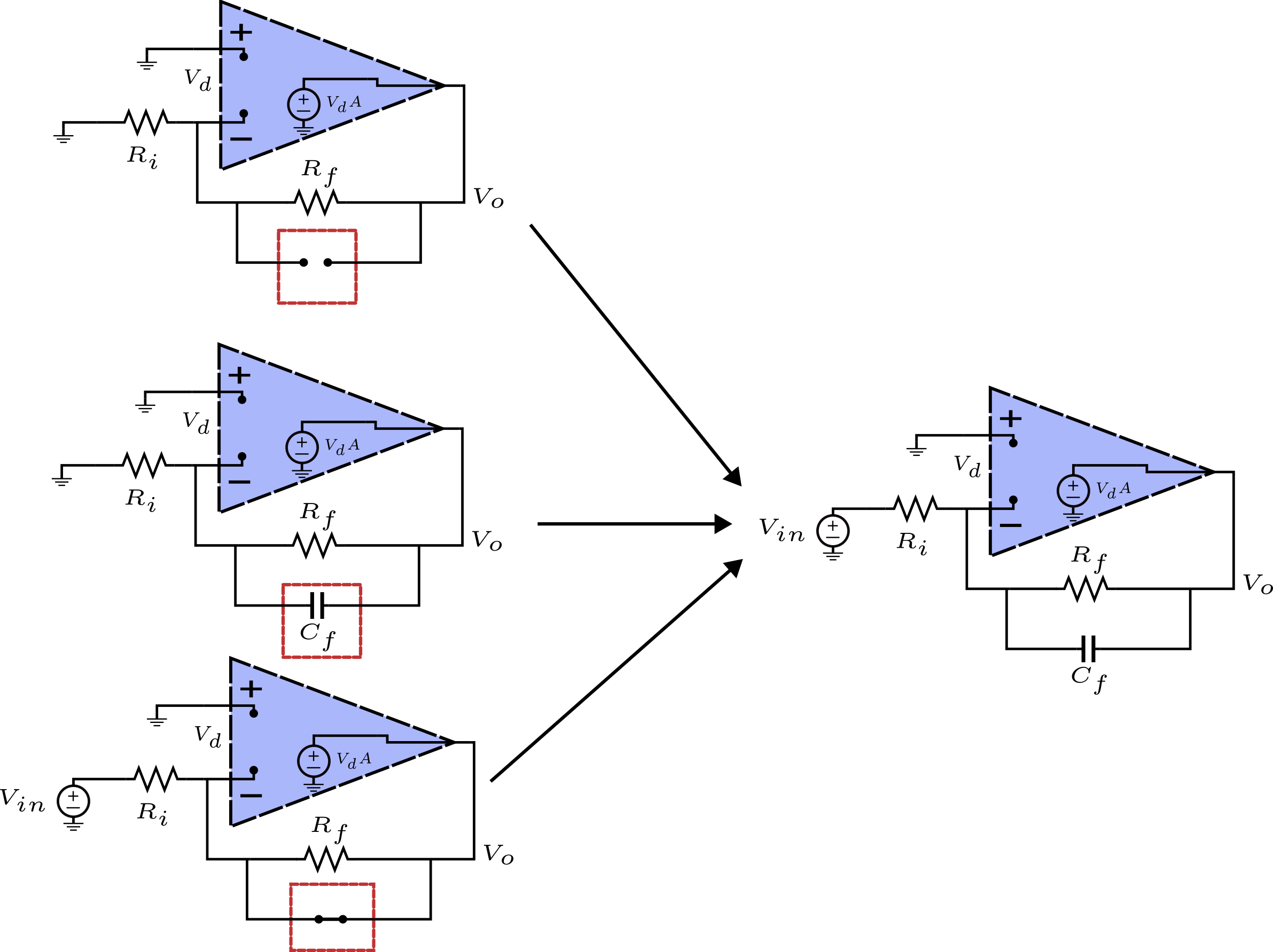
Following up with the previous article, we analyze the standard inverting amplifier with a compensation capacitor in parallel with the feedback resistor using Hajimiri’s method.
\[\begin{aligned}
H(s)=\frac{a_0 + a_1s+a_2s^2+\cdots}{1+b_1s+b_2s^2+\cdots}
\end{aligned}\]
Hajimiri’s paper already provides instructive examples of several passive and active circuits (i.e. circuits with dependent sources). This article intends to also show that this method can be applied to the analysis of op-amps, assuming a simple finite gain op-amp.
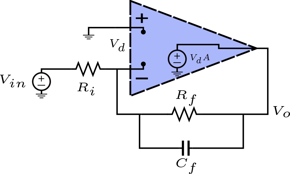
Inverting Op-Amp Closed-Loop Gain
\[\begin{aligned}
H(s)=\frac{a_0 + a_1s}{1+b_1s}
\end{aligned}\]
\[\begin{aligned}
a_0 = -\frac{R_f}{R_i}\\
b_1 = \tau_{C_f} = C_fR_f \\
a_1 = 0
\end{aligned}\]
How did we derive each term:
- \(a_0:\) This is the zero-value time constant. In this case, this equals the standard inverting op-amp transfer function.
- \(b_1:\) This term is the zero-value time constant related to \(C_f\).Under the assumption of an ideal op-amp (i.e. V(+) = V(-)), the top side of \(R_i\) is grounded as well; it’s, effectively, out of the picture. Therefore, the only resistance seen by \(C_f\) is \(R_f\). Therefore, \(\tau_{C_f}=C_fR_f\).
- \(a_1:\) This is the infinite-value transfer constant from input to output related to \(C_f\). This means, we find the trans from input to output while setting \(C_f\) to infinity (i.e., it becomes a short). When doing so, no voltage transfer is possible because the output is shorted to the input. Therefore, \(a_1=0\tau_{C_f} = 0\)
Finally, we can write the closed-loop gain formula as: \[\begin{aligned}
H(s)=\frac{-\frac{R_f}{R_i}}{1+sC_fR_f}
\end{aligned}\]
Inverting Op-Amp Loop-Gain
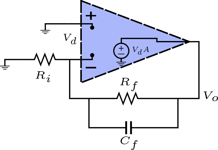
We change \(V_d\) in the controlled source by \(V_c\), so it becomes an independent voltage source now.
\[\begin{aligned}
L = \frac{V_d}{AV_c} = \frac{a_0 + a_1s}{1+b_1s}
\end{aligned}\]
\[\begin{aligned}
a_0 = \frac{R_i}{R_i + R_f}\\
b_1 = \tau_{C_f} = C_f(R_f||R_i)\\
a_1 = \tau_{C_f} = C_f(R_f||R_i)\
\end{aligned}\]
How did we derive each term?
- \(a_0:\) All dynamic elements are set to their DC value (i.e. \(C_f\) is an open). It is easy to see that the transfer from \(V_c\) to \(V_d\) is a simply voltage divider by \(R_i\) and \(R_f\).
- \(b_1:\) Since there’s only one dynamic element (i.e. \(C_f\)), we turn off all inputs (in this case, \(V_c\), which would be shorted to ground.) and simply calculate the impedance seen by \(C_f\). Since \(R_f\) is grounded on its right side, then it is effectively in parallel with \(R_i\).
- \(a_1:\) This is the transfer from \(V_c\) to \(V_d\) while setting \(C_f\) to its infinite value (i.e. a short). This renders the voltage divider due to \(R_i\) and \(R_f\) useless, as now \(R_f\) is shorted. Therefore, the transfer is simply 1. This transfer factor must be multiplied by the time constant of \(C_f\), because we infinite-valued it.
Therefore, we can write:
\[\begin{aligned}
L = \frac{V_d}{AV_c} = \frac{a_0 + a_1s}{1+b_1s} = \frac{\frac{R_i}{R_i + R_f} + sC_f(R_f||R_i)}{1+sC_f(R_f||R_i)}
\end{aligned}\]
Factoring out the constant gain term:
\[\begin{aligned}
L = \frac{V_d}{AV_c} = \frac{R_i}{R_i + R_f}\frac{1+sC_fR_f}{1+sC_f(R_f||R_i)}
\end{aligned}\]
Complete Transfer
Now, we can write the complete transfer using the asymptotic gain model:
\[\begin{aligned}
\textrm{complete transfer} = A_{\infty}\frac{-L}{1-L} = -\left(\frac{R_f}{R_i}\right) \frac{1}{1+sC_fR_f} \frac{-A\frac{R_i}{R_i + R_f}\frac{1+sC_fR_f}{1+sC_f(R_f||R_i)}}{1-A\frac{R_i}{R_i + R_f}\frac{1+sC_fR_f}{1+sC_f(R_f||R_i)}}
\end{aligned}\]